We will be amazingly imprecise in this course. One of the most difficult things that the student of physics must accept is the fact that no answer is the correct answer. We will be limited by the precision of our experiments, the sophistication of the mathematics we use to model the systems we are studying, and by the very complexity of those systems. Most of the universe is simply too complicated to treat mathematically. We will ignore most of the complexities of reality, and instead work with very simple models of the systems we study.
For instance, we will often treat extended objects as "point particles". This means we will pretend that the object has no size of its own, but still has a well-defined location, mass, charge, etc. This idealization, or simplification, allows us to ignore the internal structure of the object. As an approximation, the point particle idealization is only acceptable so long as the scale of the object's behavior is much larger than the scale of its internal structure. It may be OK to idealize a piece of chalk flying across the classroom as a point particle in order to avoid worrying about its tumbling motions, and whether it shatters when it hits the floor. But to idealize the professor stepping off a chair in that way is clearly not valid.
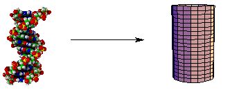
Another idealization which we will use is approximate symmetry. A long, thin object or system of objects is often sufficiently linear that it can be treated as if it were axially (cylindrically) symmetric:
The point particle enjoys spherical symmetry: all directions are equivalent with respect to a point. That is a major reason for the utility of the notion of a point particle. Similarly, round objects or systems (such as myoglobin) are often treated as if they were spheres:

Note that approximate symmetry also reduces the number of degrees of freedom needed to describe the system: a quantitative indication of the simplification.
Many times we will simply ignore the complexities of the systems we study. We will usually assume linear behavior (in the functional sense), when in fact most of the universe behaves in much more complicated fashions. We will often assume some variables to be constant (perhaps using an average value), or ignore them altogether for the sake of reducing our equations to a level which we can handle. In any event, we must always clearly document the assumptions and idealizations we make.
A common way to evaluate the quantitative behavior of a system which is too complicated to treat precisely is to compute the "order of magnitude" of one (or more) of its variables. The order of magnitude of a quantity is given by the power of ten which characterizes the scale of the quantity. For example, current estimates place the age of the universe at from 5 to 15 billion years. The order of magnitude of the age of the universe is then 10 to the 10th years: 10 billion years. Many times we will be very happy if our computational results are of the same order of magnitude as our experimental results!
At this juncture, a reminder about order of magnitude prefixes may be in order:
- k = kilo ( 10 3 )
- M = mega ( 10 6 )
- G = giga ( 10 9 )
- T = tera ( 10 12 )
- c = centi ( 10 -2 )
- m = milli ( 10 -3 )
- m = micro ( 10 -6 )
- n = nano ( 10 -9 )
- p = pico ( 10 -12 )
When dealing with experimental data, we can (and therefore must!) quantify the precision of the quantities we measure. We define the "absolute error" of a measured quantity as the difference between the average of a set of repeated measurements and the measurement farthest from the average. Statements of absolute error are often "average plus or minus absolute error". When comparing the precision of measurements of quantities with different units, we use "relative error". We define the relative error in a set of repeated measurement as the absolute error divided by the average, expressed as a percentage. Since the units of the error are the same as those of the average, the relative error is a dimensionless quantity. Note that implicit in this discussion is the fact that we must make repeated measurements of the same quantity in order to quantify the error of the measurement.
We will sometimes have to evaluate the error in a quantity which is computed from an equation involving measured quantities. This process is called "error propagation". For example, consider the following sets of measurements for the variables u and v:
| u | v |
|---|---|
| 95 | 12 |
| 100 | 15 |
| 105 | 18 |
The absolute error in u is 5 and its relative error is 5 %. The absolute error in v is 3 and its relative error is 20 %. Consider the quantity u v 2. It can range from 13,680 to 34,020. The relative error in u v 2 is 47 %! It is clear that the error has grown considerably.
For our purposes, the "root-mean-square" or "RMS" error will provide a good way to approximate the propagated error in a calculation with uncertain quantities. If A, B and C are exact quantities (ie., constants), and we are computing functions f1 and f2 from measured quantities u and v, for
the relative error in f1 is
where u rel is the relative error in u and v rel is the relative error in v. For
the relative error in f2 is
So the error in a function which is computed from uncertain quantities has a form which depends on the type of computation you are doing. The latter formula (where A is a, B is 1 and C is 2), gives a relative error for our previous example of 40%, much more in line with the error computed by hand.
See the NIST pages on constants, units and uncertainty.
The next section is about problem solving.
If you have stumbled on this page, and the equations look funny (or you just want to know where you are!), see the College Physics for Students of Biology and Chemistry home page.
©1996, Kenneth R. Koehler. All Rights Reserved. This document may be freely reproduced provided that this copyright notice is included.
Please send comments or suggestions to the author.