Our study of physics begins with the concepts of mechanics: the study of motion. We will first be concerned with kinematics, or how we describe motion. From there we will move on to the causes of motion, or dynamics. Finally, we will apply the tools we have learned to some physiological systems: biomaterials and the stresses of the skeletomuscular system. The concepts in this chapter will be used throughout the rest of the course, for they are the basis for our descriptions of motion, and what is physics if not the study of moving systems?
In order to describe objects in motion, we must first be able to unambiguously specify their position. We will typically denote position by the variable "x"; if we have more than one object to consider, we will usually add subscripts to x to indicate which object we are currently discussing. If the system we are studying lives on a plane, x will be supplemented by the variable "y". When we treat a system in all of its three dimensional splendor, we add the variable "z". Each of these variables has dimension of length, and we must carefully identify our coordinate system before using any of them.
We are all familiar with the equation for objects moving at a constant speed:
where d is distance, r is rate or speed, and t is the time. Indeed, this is often the only equation the typical student can recall from their algebra course. We can alter that equation to define the average speed as
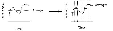
where the Greek letter D (capital "delta") denotes a finite change in the quantity which follows. In this case, Dx denotes a finite distance (d in the previous equation), and Dt denotes a finite time interval (t in the previous equation). The speed thus defined is a time average: we can only say that during the time interval Dt, the object moved with average speed s.
The language of calculus was created to deal with physical systems whose parameters change constantly. We will not use calculus in this course, but we will use some of its notation to denote instantaneous rates of change. An instantaneous rate of change is obtained when we make the time interval Dt infinitesimal; that is, as the time interval gets smaller and smaller, the average value of the speed gets closer and closer to the instantaneous value at that instant:
Such an instantaneous rate of change is called a "derivative", and is denoted
The instantaneous rate of change of position is called the "velocity":
The dimension of velocity is still the expected length divided by time; the notion of speed is the same, but it is now an instantaneous value instead of a time average.
We can also speak of the instantaneous rate of change of velocity, or "acceleration":
The dimension of acceleration is length divided by time squared. We will often deal with systems whose acceleration is a constant with respect to time. Near the surface of the Earth, we treat gravity that way: "g" is the acceleration due to gravity, and is assumed to be essentially constant with a value of 9.8 m / s 2. Note that this is one of our idealizations: we ignore the variability of g in order to be able to treat the system mathematically more easily. For such a system, the position is given by
Here the zero subscripts (read "nought") indicate the initial position and velocity of the object. By borrowing a simple formula from calculus for the derivative of a polynomial term
we see that
and
So the equation does indeed describe a object undergoing uniform acceleration.
Uniform acceleration is often used as a first approximation in analyzing collisions. Consider an automobile accident in which the driver's head hits the windshield. The initial velocity of the head is the same as that of the car before the accident, and the acceleration is negative (it "decelerates") since the head slows to rest, losing velocity. We assume that the deceleration is constant since we do not know how it varies with time. The position equation
and its companion
represent two equations in six unknowns (x, v, t, x 0, v 0 and a) and can be solved for any two of them, given the other four. Note that the final velocity v is zero due to the nature of the situation.
For instance, assume that the initial velocity is 11 m / s and the driver's head comes to rest 3 ms after first touching the windshield. We find that the deceleration is almost 3700 m / s 2! This seems very large, but is in fact typical of sudden collisions. Often we do not need to know exactly where the object stopped, but rather how far it travelled while it was slowing down. From the first equation, we find that x - x 0 is 1.65 cm.
Notice, however, that given other facts about the collision, we can compute what was given above. For instance, assume that the driver's head came to rest after travelling 2 cm, and that the deceleration was measured (somehow without measuring the velocities and elapsed time!) to be 4000 m / s 2. Now the problem is a little tougher, at least algebraically. Even though we do not know the initial velocity, we can use the velocity equation to express it in terms of the acceleration and the elapsed time:
After substituting, this gives us
or
From this, we find that t is 3.2 ms, and that the initial velocity was 12.65 m / s. You will often want to use this trick while practicing your problem solving skills: any problem which you have already solved one way becomes a different problem when you exchange the givens and the unknowns.
There is one more kinematic quantity that will be very useful to us. We define the "kinetic energy". or energy of motion, of a moving object as
where m is the mass of the object and v is its velocity. Kinetic energy has dimensions of mass times length squared over time squared, and its SI unit is the "Joule":
The cgs unit of energy is the "erg":
Note that kinetic energy is always positive, since mass is always positive, and the square of any quantity (ie., velocity) is as well.
The next section is an interlude on vectors.
If you have stumbled on this page, and the equations look funny (or you just want to know where you are!), see the College Physics for Students of Biology and Chemistry home page.
©1996, Kenneth R. Koehler. All Rights Reserved. This document may be freely reproduced provided that this copyright notice is included.
Please send comments or suggestions to the author.