Electric Potential

Now that we have some understanding of the nature of the electrical force, we can ask a few more fundamental questions: why is it proportional to the product of the charges? Why does its strength depend inversely on the square of the separation? Can we develop a model for the electrical "influence" of a single isolated charge, when there are no other charges nearby to interact with it?

Physicists attempt to work with as few assumptions as possible. One of the fundamental assumptions is that the interactions of two distinguishable objects are independent of the labels we use to identify them. Hence the electrical force between two charges must be the same regardless of which we call q₁ and which is called q₂. The equation for force must therefore be "symmetric" under exchange of the labels: the value of the force must be the same. This means that the force can only depend on the sum or the product of the charges; experiment tells us that it is the product.

In order to model the electrical influence of an isolated charge, we resort to a rather fictional scenario. We first "fix" (think of it as glueing) a charge (or charges) at specific coordinates in space. This charge is called the "configuration charge". We think of the configuration charge as the source of an "electrical field", which has a different magnitude and direction at every point in space:

where the subscript "c" on the charge indicates that it is a configuration charge. Here, r as the argument of the function E specifies a location (the "field point") where we want to compute the field; r in the denominator specifies the distance from the configuration charge to the field point, and R is the vector pointing from the configuration charge to the field point. This electric field has dimensions of force over charge, and the force felt by a "test" particle in this field is

("t" indicating a test charge) which is equivalent to the Coulomb force. The notion here is that a charged particle has an influence independent of whatever forces are felt by other charges. Since the electric field is a vector, linear superposition again applies: the electric field at any given point in space due to a sum of configuration charges is equal to the sum of the electric fields at that point. Note that the field concept is a model: the field is not measurable independently of the force. That, however, is not the fictional part of the story: we pretend that the test charge DOES NOT INFLUENCE the electrical field created by the configuration charges. Since the configuration charges are "static" (do not move), they are the sources of the "electrostatic field"; the test charge is a probe which does not affect that field. In other words, it is an idealized measuring device with which we determine F (and therefore E) due to the charge configuration.

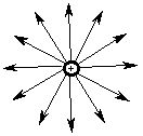
If we want a picture of a field, we usually think of many lines of "flux" emmanating radially away from the charge:

For negative charges, the lines point inward. These flux lines indicate the direction a positively charged test particle would move due to the electric force between it and the configuration charge. The "number" of lines is proportional to the quantity of the configuration charge. Note that the "density per unit area" of the flux decreases as the distance from the center increases. That is, the lines are much closer together when nearer to their origin. Since we live in three spatial dimensions, and the surface area of a sphere centered on the charge increases with the square of the distance, we have a model for the inverse square force law: the magnitude of the force is proportional to the density of the field lines ("flux density"), which decreases with the square of the distance. We can also see why a spherical source is equivalent to a point source at its center: the flux lines emanating from the surface can be extrapolated inwards to the center with no change in the physical forces felt outside the surface.

With the concept of an electric field we can now understand the idea behind electrophoresis. Electrophoresis is a sedimentation technique used in DNA analysis and the determination of protein molecular weights, but one in which the force of gravity (or the centrifugal force induced by a centrifuge) is replaced by the electric force. The sample to be analyzed is placed along one end of a gel (whose diffusion properties are very carefully controlled) and an electric field is created whose magnitude is constant and whose direction is along the gel and perpendicular to the sample. Since the electric force is much larger than that of gravity, we can ignore gravity and equate the force experienced by the sample molecules to the difference between the electric force and the drag:

where q is the charge on the molecule and b is its drag coefficient. The molecules rapidly reach terminal velocity:

and the measurement of the velocity (or correspondingly, the distance the molecules travel in a given time) determines the charge on the molecule. Provided that the molecules have been denatured (unfolded) and charged by the addition of an anionic detergent like sodium dodecylsulfate (SDS), the charge will be proportional to the mass of the molecule and the molecular weight can be determined. This molecular weight is relative to an accurately calibrated standard, since the charge to mass ratio and the drag coefficients cannot be controlled sufficiently accurately to enable the molecular weight to be computed directly from the position. In practice, the sample is first spread by electrophoresis into a thin line at one end of the gel, which is manufactured with a pH gradient along that direction. Since the mobility of each molecule is a function of the pH, each molecule will stop moving at the point where it is electrically neutral relative to the surrounding pH (its "isoelectric" point). Then the sample is subjected to an electric field perpendicular to the line; thus electrophoresis yields a two dimensional "map" of the sample, with different proteins (or DNA sequences) separated by molecular weight. These maps are what you worked with in problem 2-12.

For our purposes, it will be much easier to deal with another quantity, the scalar "electrical potential", rather than the electric field. The electric field can be thought of as the gradient of the electrical potential field. This notion is identical to the notion in Chapter 2 of the force as the gradient of the potential energy function. But since the electric field is a force per unit charge, the electric potential must be an energy per unit charge. It is a scalar field, having a magnitude (but no direction) at every point in space:

It has SI units of J / C ("Volts"), and the energy of a test charge in the potential field due to one or more configuration charges is

The electric (or "electrostatic") potential is analogous to temperature: there is a different temperature at every point in space, and the temperature gradients tell you where heat flows. Similarly, there is an electric potential at every point in space, and its gradient (the electric field) tells you where charges move.

As with the cases of the electric field and force, the electrical potential field superposes linearly, so that the field at a point due to a collection of configuration charges is equal to the sum of the fields due to the individual charges, at that point. For example, if in a vacuum two protons (q _{c 1}) lie in the xy plane at (x ₁, y ₁) = (-2,1) Angstroms and an electron (q _{c 2}) lies at the origin ((x ₂, y ₂) = (0,0)), the energy of an electron (q _t) at (x _t, y _t) = (1,1) Angstroms would be

U = U _{t c1} + U _{t c2}

(= q _t (V_{c 1} + V_{c 2}))

= (- e) (2 e) / (4 p e₀ 3 x 10^{- 10}) + (- e) (e) / (4 p e ₀ Sqrt (2) x 10^{- 10})

and "i" denotes either of the configuration charges. Note that chemists often compute energies in kJ / mol, which would necessitate multiplying the above answer by a conversion factor of N _A / 1000.

In order to compute the direction of the force felt by a test charge in a potential field, one can take the gradient of the potential

and then compute the force as above. There is, however, an easier way. If we were to plot the electrical potential field due to a pair of configuration charges, we would see that there are lines, called "equipotentials", on which the electrical potential has the same value everywhere:

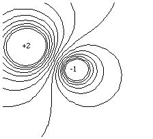
The direction of the gradient (and hence the electric field) is perpendicular to the equipotential lines since its component along (tangent to) the equipotentials is zero (V is a constant). We can therefore immediately trace the path of any test particle in the field, since charges move in the direction of least energy. The force it experiences is equal to the product of its charge and the electric field it is in, so the particle moves along the gradient, perpendicular to the equipotentials:

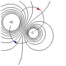
Here the blue line represents the motion of a negative test charge, and the red line represents the motion of a positive one. Try the Java simulation of a proton in a potential field. Note that while the initial motion is perpendicular to the equipotentials, the buildup of momentum also affects the trajectory!

In the case of electrophoresis, the constant electric field is created by establishing a potential which varies linearly with the distance along the gel. Luckily, this is easy to do.